Data Preprocessing

Data Preprocessing in Machine Learning 🧠

machine learning models only look smart if you feed them good data. And most data in the real world is, frankly, a mess missing values everywhere, weird formats, numbers and text all jumbled up. That’s why data preprocessing is a big deal.

Think of preprocessing like prepping your ingredients before you cook. Even chefs can’t save a meal if the veggies are dirty or the chicken isn’t cut right.

Here’s what we’ll cover in this guide (github repo at very bottom btw!):

Why preprocessing actually matters
The steps you should follow
How to deal with missing data
Turning text into numbers (the easy way)
Why train/test splits are crucial
When to use fit() vs. transform()
Should you use Standardization or Normalization?
Full, copy-ready code examples

What Is Data Preprocessing?

Data preprocessing is the set of steps you use to turn ugly, messy datasets into clean and tidy numbers so your machine learning model doesnt freak out. If you skip this stuff your model will potentially either fail or just learn nonsense.

messy data usually has stuff like:

missing values
text columns that need converting to numbers or binary
widly different ranges of numbers (like “Age” 1–90 and “Salary” 20,000–200,000)
different types mixed together (strings, integers, floats)
Outliers
Columns you don’t need

Preprocessing makes sure your data is actually usable and gives your algorithm a refined dataset to learning something.

The Standard Machine Learning Preprocessing Pipeline

here is the standard preprocessing pipeline 1. Import libraries 2. Import the dataset 3. Fix missing data 4. Encode categorical features 5. Split into training & test sets 6. Scale your features

This might look simple, but each step has some real logic behind it. Let’s break them down! also we some best libraries for machine learning is sci-kit learn, pandas, numpy and matplotlib which we will be using them later... not important for now but just cuz uk

Types of Variables

In any dataset, you’ll find two main kinds of columns:

Feature variables (independent variables): These are all the inputs or properties the things you use to help predict something else.
Target variable (dependent variable): This is what youre trying to predict or explain. The model looks at the features to learn patterns and figure out this target.

Handling Missing Data

missing values are normal in real data, but ML algorithms hate them.

Three main ways to deal with them:

1. just remove them

you can remove them but do this whenever u feel like there is barely any row missing cuz if u remove max portion then its just pointless

2. Fill Them In (“Impute”)

This is what people usually do.

numerical columns:(age, salary) fill with median or mean
category columns:(gender, caste!!) fill with the most frequent value

Text

from sklearn.impute import SimpleImputer
import numpy as np

num_imputer = SimpleImputer(strategy="median")
cat_imputer = SimpleImputer(strategy="most_frequent")

df[num_cols] = num_imputer.fit_transform(df[num_cols])
df[cat_cols] = cat_imputer.fit_transform(df[cat_cols])

Encoding Categorical Data

Algorithms can’t handle words or text—they only work with numbers. So, we need to “encode” categories.

Label Encoding

Simply gives each category its own number (also its only valid for dependent variable)

Color	Encoded
Red	0
Blue	1
Green	2

Only use label encoding if the categories have a natural order (like Low < Medium < High).

One-Hot Encoding (Most Common and used for feature variable)

Turns each category into a brand-new column that’s either 1 or 0.

Sex	Sex_Male	Sex_Female
male	1	0
female	0	1

This is almost always better for things like city, gender, country, etc.

A ColumnTransformer in scikit-learn helps automate this (just pass it a list of categorical columns):

Text

from sklearn.preprocessing import OneHotEncoder
from sklearn.compose import ColumnTransformer

ct = ColumnTransformer(
    transformers=[("encode", OneHotEncoder(), ['Gender','City'])],
    remainder='passthrough'
)

X = ct.fit_transform(X)

why is it important to split the dataset into training and test sets?

Honestly, this step is misunderstood by almost everyone starting out, but it’s super important.

💡 1. It’s How the Real World Works

The “test” set acts like totally new data—it helps you see if your model would actually work out in the wild.

💡 2. Stop the Model From Just Memorizing

If you train AND test on the same data, your model will just memorize stuff, look “perfect”—but it’ll fail when it sees new data.

💡 3. Honest, Fair Evaluation

By keeping the test data separate, you’re not “cheating.” Your accuracy is real, not just wishful thinking.

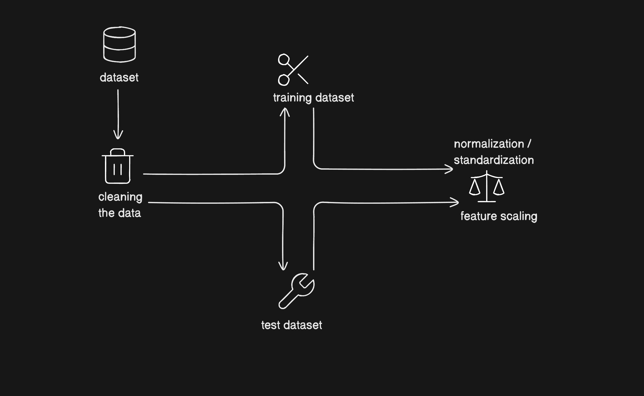
Typical train/test splits

80% train / 20% test
70% train / 30% test
For classification tasks, always use stratify=y so that the class ratios stay similar in both sets.

Text

from sklearn.model_selection import train_test_split

X_train, X_test, y_train, y_test = train_test_split(
    X, y, test_size=0.2, random_state=42, stratify=y
)

Feature Scaling — Normalization vs Standardization

keep in mind this step is very optional from models to models and u should only execute it after splitting the datasets Some models get messed up if your features are on totally different scales.

Example:

Age ranges from 0 to 100
Salary ranges from 20,000 to 200,000

If you don’t scale, salary ends up “dominating” the model just by being bigger numerically.

Standardization (Z-score scaling)

Text

x_standard = (x - mean) / standard_deviation

What happens?

The mean becomes 0
The standard deviation is 1

Use standardization when you’re working with anything its reliable anywhere and everywhere

Text

from sklearn.preprocessing import StandardScaler

scaler = StandardScaler()
X_train_scaled = scaler.fit_transform(X_train)
X_test_scaled = scaler.transform(X_test)

Normalization (Min-Max scaling)

Text

x_norm = (x - min) / (max - min)

Everything gets squeezed into the 0–1 range.

Best for:

Neural networks / deep learning
When features need to be bounded

Text

from sklearn.preprocessing import MinMaxScaler

scaler = MinMaxScaler()
X_train_scaled = scaler.fit_transform(X_train)
X_test_scaled = scaler.transform(X_test)

Why Use `fit()` on Training Data, But Not Test Data?

This is one of the golden rules of ML.

`fit()` = learn from training data

Learns mean & std for scaling
Remembers which categories exist
Stores imputation values

`transform()` = applies what it learned

Don’t “fit” on test data! Why?

You’d be “peeking” at answers you shouldn’t see
It lets info leak from test to train, messing up real-world performance
Your accuracy scores will be unrealistically high

So do it like this:

Text

scaler.fit(X_train)       # learn from train data
scaler.transform(X_train) # scale train
scaler.transform(X_test)  # scale test (no fitting!)

Full Example Pipeline (Best Practice)

Check out how to tie it all together using scikit-learn pipelines:

Text

from sklearn.pipeline import Pipeline
from sklearn.compose import ColumnTransformer
from sklearn.impute import SimpleImputer
from sklearn.preprocessing import OneHotEncoder, StandardScaler

num_cols = ['Age', 'Salary']
cat_cols = ['Country', 'Gender']

num_pipeline = Pipeline([
    ('imputer', SimpleImputer(strategy='median')),
    ('scaler', StandardScaler())
])

cat_pipeline = Pipeline([
    ('imputer', SimpleImputer(strategy='most_frequent')),
    ('encode', OneHotEncoder(handle_unknown='ignore'))
])

preprocessor = ColumnTransformer([
    ('num', num_pipeline, num_cols),
    ('cat', cat_pipeline, cat_cols)
])

X_train_prep = preprocessor.fit_transform(X_train)
X_test_prep  = preprocessor.transform(X_test)

This is basically how things are done in the real world—not just in tutorials!

Final Thoughts: Preprocessing Isn’t Optional

You don’t need the fanciest model to get great results. What you do need is clean, well-prepped data.

When you:

handle missing values
encode categorical features
scale your numbers
split your data the right way
and avoid any data leaks

…your model becomes more accurate, stable, and realistic.

here are the resources and codebases all required

👉 https://github.com/Proxyy587/ml-ops

If this was helpful, feel free to star the repo or subscribe to rss along for more updates

Data Preprocessing